
Introduction
In this instalment of our blog series focusing on the multi-curve framework in the OpenGamma Strata library, we will discuss the impact of interpolation on forwards and on the delta risk. The goal of the blog is to show a couple of examples and provide a code base for the readers to reproduce and expand those examples. The code can be found on the Strata GitHub repository here.
One important point in the discussion on interpolation in interest rate curve, before the question on how to interpolate should be the question of What to interpolate? I do not plan to discuss that issue in this blog, but you can find my rant on the subject in Section 4.1 of my book on the multi-curve framework (Henrard (2014)). In this blog, I have decided to use interpolation on the zero-rate (continuously compounded), which is probably the most used approach
We start with the graphical representation of impact of interpolation. For this I use that same data as used in the previous blog, calibrating two curves in GBP to realistic market data from 1-Aug-2016. One curve is the OIS (SONIA) curve and the other one is the forward LIBOR 6M curve. The nodes of the curves are the node prescribed by the FRTB rules (see BCBS (2016)). Similar effects would be visible with roughly any selection of node; they were selected for convenience.
We will use through this blog three types of interpolation schemes: linear, double quadratic and natural cubic spline. The reason for the choice is to have interpolation schemes with different properties, I do not claim that those are the best for all (or even any) purposes. The graph of the forward Sonia rates, daily between the data date and 31 years later is displayed in Figure 1. Each date is represented by one point.
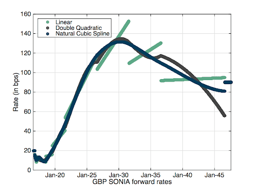
Figure 1: Overnight forward rates with three different interpolators.
The forward rates for the Libor curves are provided in Figure 2.
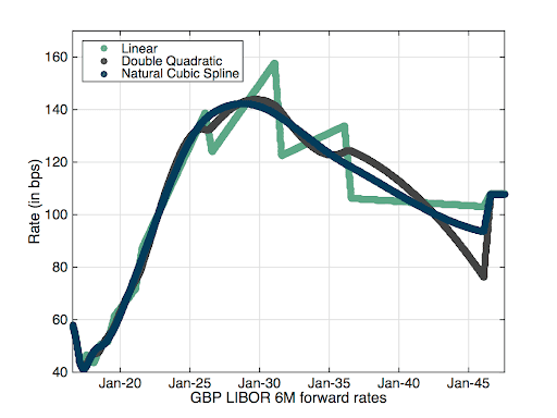
Figure 2: Libor 6M forward rates with three different interpolators.
The graphs are like the familiar one on any note related to curve interpolation. The linear interpolation leads, even with very clean data like in this example, to forward rates profiles with saw tooth effect. Some impacts are very pronounced; in the middle of the graph there is a drop of 40 bps in forward rate from one day to the next. An almost similar drop if visible in the Libor graph, but this time on a period of 6 months (one tenor of the underlying Libor). There is also a large difference between the different interpolators. In the case of the overnight rates, the largest difference in forward rate is 39.29 bps and is observed for the rate starting on 31-Jul-2046 (30 years forward) between the linear and the double quadratic.
The code used to produce the above graphs are available in the blog example Strata code [link]. The code to produce the above curves is roughly 10 lines. The code to export the data to be graphed by Matlab is longer than the calibration code itself.
The interpolation mechanism does not only have an impact on the forward rates, and thus on the present value, but also on the implied risk. We now look at this risk, using the bucketed PV01 or key rate duration as the main risk indicator. For this we take one forward swap with starting date in 6 months and a tenor of 9 years. The fixed rate is 2.5% (above market rate). For that swaps, the par rate bucketed PV01 are provided in Figures 3 to 5.
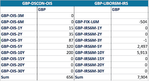
Figure 3: PV01 with linear interpolation scheme

Figure 4: PV01 with double quadratic interpolation scheme
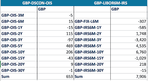
Figure 5: PV01 with natural cubic spline interpolation scheme
The first point to notice is that the sum of the bucketed PV01 for both the OIS curve and the Libor curve are almost the same for all interpolation schemes. A parallel curve move results in similar change of PV and there is only a very small effect from the level and the curve shape.
The interesting part is obviously the differences. The double quadratic and natural cubic spline are non-local interpolators. The sensitivity to the cash flows in the 5Y to 10Y period extend beyond the 5Y and 10Y nodes. There is a sensitivity to the 3Y and 15Y points, and in the case of the natural cubic spline (NCS), even to the 20Y and 30Y points. The non-locality can lead to non-intuitive hedging results. In the NCS case, the hedging of the swap with a maturity of 9Y and 6M is done with swap up to 10Y but also with swaps of maturity 15Y, 20Y and 30Y. Note also the “wave” effect where the hedging is done alternatively with swap of the opposite direction as the original one and the same direction.
The code to calibrate the three sets of curves and computing the related par market quote sensitivities – the variable mqs in the code – takes only 10 lines:
/* Calibrate curves */ ImmutableRatesProvider[] multicurve = new ImmutableRatesProvider[3]; for (int loopconfig = 0; loopconfig < NB_SETTINGS; loopconfig++) { multicurve[loopconfig] = CALIBRATOR.calibrate(configs.get(loopconfig).get(CONFIG_NAME), MARKET_QUOTES, REF_DATA); } /* Computes PV and bucketed PV01 */ MultiCurrencyAmount[] pv = new MultiCurrencyAmount[NB_SETTINGS]; /* Computes PV and bucketed PV01 */ MultiCurrencyAmount[] pv = new MultiCurrencyAmount[NB_SETTINGS]; CurrencyParameterSensitivities[] mqs = new CurrencyParameterSensitivities[NB_SETTINGS]; for (int loopconfig = 0; loopconfig < NB_SETTINGS; loopconfig++) { pv[loopconfig] = PRICER_SWAP.presentValue(swap, multicurve[loopconfig]); PointSensitivities pts = PRICER_SWAP.presentValueSensitivity(swap, multicurve[loopconfig]); CurrencyParameterSensitivities ps = multicurve[loopconfig].parameterSensitivity(pts); mqs[loopconfig] = MQC.sensitivity(ps, multicurve[loopconfig]); }
It is also interesting to look at a “dynamic” version of the above PV01 report. For that I will produce the same report for swaps with starting dates between the data date and two years later and all of them with a tenor of 8 years. The swap maturities will be between 8 years and 10 years. Let’s start with the linear interpolation scheme as it displays the profile that most people would probably consider as intuitive (at least I do). That profile is displayed in Figure 6. For a 8Y spot starting swap (the left side of the graph), the sensitivity is mainly on the 5Y and 10Y IRS with more on the 10Y. The main sensitivities are represented by the colour curves; the other sensitivities (Libor and OIS) are represented by the dark grey thin lines. When we move to the 2Yx8Y swap along the X-axis, we see the sensitivity to the 10Y increase and the sensitivity to the 5Y decrease down to zero. The sensitivity to the 2Y increase in absolute value but with the opposite sign to the 10Y. The total sensitivities of the swaps are fairly constant.
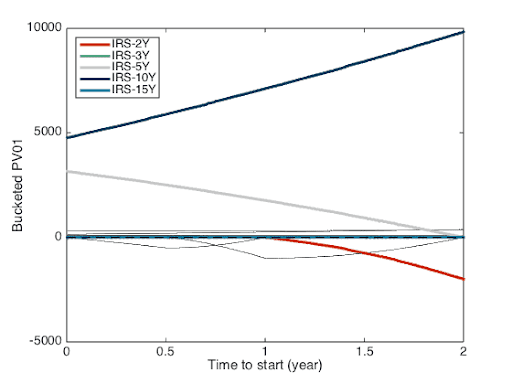
Figure 6: PV01 profile for linear interpolation scheme.
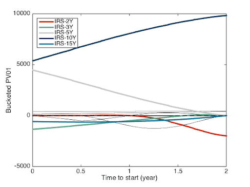
Figure 7: PV01 profile for double quadratic interpolation scheme.
Let’s jump immediately to the natural cubic spline profile displayed in Figure 8; the Figure 7 for double quadratic is in between the other two. For that profile, I will start the explanation from the right side, with the 2Yx8Y forward swap. The risk is very similar to the one depicted by the linear interpolation. The main sensitivities (2Y and 10Y) are on nodes and the sensitivity in the two cases are similar. When we move away from the nodes, in our case with the starting date moving down from 2Y to valuation date and the maturity from 10Y down to 2Y, a different profile appear. Sensitivities are not anymore only to the nodes surrounding the swap dates. There are now significant sensitivities to the adjacent nodes (3Y and 15Y for example) with the opposite sign to the main sensitivities with a non intuitive behavior. For example the sensitivity to the 15Y node increases when the maturity of the swap moves away from that node. A significant sensitivity appear on the 2Y when the start date of the swap moves away from the 2Y node and is the larger in this profile for the spot starting swap.
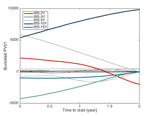
Figure 8: PV01 profile for natural cubic spline interpolation scheme.
Obviously the sensitivity to different nodes will lead to recommended hedging using swaps with those tenors. The 8Y swap will be hedged with 2Y, 3Y, 5Y, 10Y and 15Y swaps. Maybe not the most intuitive approach. It is also possible to easily compute the require notional to hedge each sensitivity, and that will be described in a forthcoming instalment of this blog.
The goal of this blog was not to provide a definitive answer on which interpolation scheme to use for curve calibration – I don’t with there is such a definitive answer – but to show that a personal analysis is important. The analysis can be done easily with the right tools. The code used to produce figures 3 to 5 is available in the examples associated to this blog. The main part of the code consists in roughly 10 lines of code, for calibration and sensitivity computation. The other figures required a loop around that code to produce the sensitivities for roughly 500 swaps (2Y of business days).
In this instalment of the multi-curve blogs, we have provided some example of interpolation impact on forward rate and risk computations. We also showed how easy it is to obtain those results in the Strata code.
References
Henrard, M. (2014). Interest rate modelling in the Multi-curve Framework: Foundation, Evolution and Implementation. Palgrave.
BCBS (2016). Minimum capital requirements for market risk. Basel Committee on Banking Supervision, January 2016.